Articulatory synthesis

This page describes my contributions to articulatory synthesis of human speech. You can download Matlab scripts here. More details are available in publications [1-4]. Articulatory synthesis consists in numerically simulating the articulatory and aeroacoustic phenomana involved in speech production. A complete articulatory synthesizer requires fine modelings of the speech production at several levels, as shown in Fig. 1

ArtSynthSchema — Fig1. - Diagram representing the different modeling levels required for a complete articulatory synthesizer

- The temporal evolution of the vocal tract geometry is driven via an articulatory model. It defines the position and deformations of the articulators (lips, tongue, larynx, velum...) using a small amount of parameters.
- The voice source is generated via a glottis model, which should be designed so that it reproduces the self-oscillating movements of the vocal folds, as well as their abduction and adduction movements.
- A synthesizer, which is a solver of the equations driving the acoustic propagation of the phonatory source through the vocal tract, generates the acoustic output, namely the synthesized speech signal.

Acoustic propagation inside the vocal tract seen as a waveguide network

The acoustic propagation is computed thanks to the Transmission Line Circuit Analog model (TLCA), proposed by Maeda [5]. This paradigm uses a spatially sampled vocal tract: the latter is seen as a 1-D waveguide with variable section, made up by elementary cylindrical tubes, or tubelets, having dimensions that approximate the the vocal tract geometry. Then, it is based on the electric-acoustic analogy: tubelets are modeled as lumped circuit elements, as shown in Fig. 2. The choice of TLCA models is motivated by the fact that, unlike its main concurrent paradigm, the Reflection Type Line Analog model (RTLA) [6], it can easily deal with time-varying shapes of the vocal tract. Hence an adequat use with realistical anatomic data of the vocal tract.

Such an analogy enables the acoustic equations to be written into a matrix form $\mathbf{f}=\mathbf{Zu}$, where $\mathbf{f}$ is a vector containing the pressure forces inside each tubelet, $\mathbf{Z}$ is a tridiagonal square matrix containing the impedance and acoustic loss terms associated with each tubelet, and $\mathbf{u}$ is the solution vector containing the volume velocities inside the tubelets. At each simulation step, the linear system of equations is solved from the knowledge of $\mathbf{f}$ and $\mathbf{Z}$, defined by the area and the length of the different tubelets.

Since we want to deal with realistic geometries of the vocal tract, side cavities, including nasal tract, piriform fossae, bilateral channels, and so on, should be simultaneously considered during the simulation. Mokhtari et al. [7] have recently proposed a generalization of the matrix formulation by Maeda for a waveguide network. It consists in the concatenation of the linear systems governing the acoustic propagation inside each individual side branch, with the addition of coupling submatrices to consider the kind of connection between the side branches:
$$\left[\begin{array}{c}\mathbf{f}^{(1)} \\ \mathbf{f}^{(2)} \\ \vdots \\ \mathbf{f}^{(\mathcal{N})} \end{array}\right] = \left[\begin{array}{cccc} \mathbf{Z}^{(1)} & \mathbf{C}_1^{(2)T} & \ldots & \mathbf{C}_1^{(\mathcal{N})T}\\ %\hline \textbf{C}_1^{(2)} & \textbf{Z}^{(2)} & & \\ \vdots & & \ddots & \\ \mathbf{C}_1^{(\mathcal{N})} & & & \mathbf{Z}^{(\mathcal{N})} \end{array} \right].\left[\begin{array}{c}\textbf{u}^{(1)}\\ \textbf{u}^{(2)} \\ \vdots \\ \mathbf{u}^{(\mathcal{N})} \end{array}\right],$$
where $\textbf{C}_m^{(n)}$ is the coupling submatrix that defines the coupling between waveguide $m$ and waveguide $n$. The generalization by Mokhtari of the matrix formulation to $\mathcal{N}$ waveguides with variable section considers 3 kinds of coupling:
1. side branches $m$ and $n$ are not directly connected, then $\textbf{C}_m^{(n)}=\mathbf{0}$
2. side branch $n$ is connected to its parent $m$ at one point (the nasal tract, for instance, which is connected to the oral tract at the velum).
3. two side branches are connected to the same parent at the same point (case of the piriform fossae, for instance, which are connected to the oropharynx at the same position).

My work on the subject allowed a fourth kind of relationship to be added to the single matrix formulation. It is the case of bilateral channels, namely the occurence of a local division of the main air path into two paralllel channels due to an obstacle. In speech production, this occurs during the pronounciation of lateral consonants, such as /l/: the air flow is divided into lateral channels that go through both sides of the tongue. This contribution enables the acoustic clues of bilateral conditions, such as the introduction of a zero due to the asymmetry of the lateral channels [8], to be simulated in the context of continuous speech synthesis. Fig. 3 shows the transfer functions of several asymmetric configurations of bilateral channels computed via our method. It highlights the appearance of a pole/zero pair due to the asymmetry factor. The frequency of the zero agrees with the theoretical frequency (red circles).

Fig3. - Left: simplified representation of the vocal tract during the pronunciation of bilateral /l/, after [9]. Note that the tongue also forms a supralingual cavity, which introduces also a zero in the transfer function (here around 2700 Hz). Right: Transfer functions of the vocal tract as a function of the asymmetry ratio of the bilateral channels. Top curves: high asymmetry ratio (1.37). Bottom curves: low asymmetry ratio. Theoretical positions of zeros are marked by red circles.

The acoustic equations have also been slightly modified to support the integration of a self-oscillating model for the glottal source. This introduces a quadratic term to account for the pressure drop inside the glottal constriction. Fig. 4 shows simulations of sustained French vowels obtained with the waveguide network paradigm connected to a classic $2\times2$ mass-spring model with smooth contours and a mobile separation point. Such simulation framework is then a useful tool to study the condition of vocal folds oscillations (or voicing production) in the context of continuous speech. Fig. 4 also shows that, compared to other classical methods, it generates similar resonance frequencies than the compared methods. It can then be used for natural speech synthesis.

Fig4. - a) Simulations of sustained French vowels (left: /a/, right /i/). From top to bottom : spectrum and spectral envelope (red), output pressure, glottal flow, and height opening of the vocal folds.

b) Formant frequencies generated with 3 methods for 6 different French vowels. Our method (ESMF) generates formant frequencies very close to the one generated via the reference frequency-based method CMP.

A glottis model to generate the acoustic source

My works on the glottis modeling focuses on the consideration of partial glottal closure. In some cases, as for the production of voiced fricatives, or breathy voices, only a portion of the vocal folds are vibrating, the other part is partially abducted. As a consequence, a triangular chink appears in the glottis shape, causing a air leakage, as shown in Fig.5 a). Classic lumped mass-spring models of vocal folds [10-12] do not consider this case. In [1-2], I proposed to overcome this limitation by allowing a constant air flow to be taken into account in parallel to the vocal folds oscillations. In the electric-acoustic analogy (see Fig. 5), the glottis is then modeled as two parallel branches, a first one accounting for the oscillating portion of the vocal folds, and the other one corresponding to the air leakage through the glottal chink.

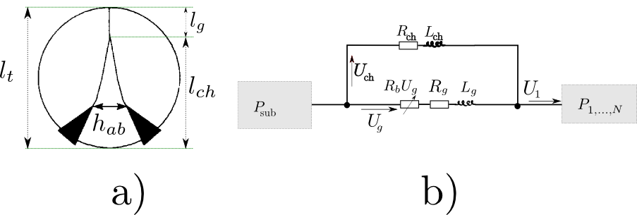
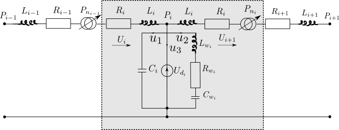
Fig5. - a) Top view of the glottis model: the upper part of the vocal folds, having length $l_g$, behave in a nominal way, while the anterior part, having length $l_{ch}$ is constantly open, due to the partial abduction $h_{ab}$ of the vocal folds. b) Electric-acoustic analogy of the glottis model: the glottal chink is characterized by a side branch, parallel to the self-oscillating branch.

Equations driving the aeroacoustic conditions around the glottis are slightly modified to consider the parallel branch due to the glottal chink opening, hence the following formulation of the system of equations
$$\left[\begin{array}{c}\mathbf{f}^{(1)} \\ F_{ch} \end{array}\right]=\left[\begin{array}{cc} \mathbf{Z}^{(1)} & \mathbf{C}_{1}^{(ch)T} \\ \mathbf{C}_{1}^{(ch)} & Z_{ch} \end{array}\right].\left[\begin{array}{c}\mathbf{u}^{(1)} \\ U_{ch} \end{array}\right]+R_bU_g^2,$$
where $Z_{ch}$ is the term accounting for the chink impedance, $U_{ch}$ and $U_g$ are the volume velocities through the chink and the vocal folds, respectively, and $R_b$ is the Bernoulli term accounting for the pressure drop inside the glottal constriction. It only depends on the geometry of the glottal constriction.

Fig. 6 shows a simulation of a sustained /i/ with a variable chink length. The opening of the glottal chink leads to a DC component of the glottal flow. Here is a video showing the movements of the vocal folds, modeled as a 2$\times$2 mass self-oscillating system during the simulation. They are displayed in details in the top left plot. The top-center plot shows the pressure distribution along the vocal tract. Bottom-left plot is a top view of the vocal folds, with the appareance of the glottal chink at the bottom, and the center plot is the position of the 2 masses modeling the vocal folds as a function of time. The right column displays the elements of Fig. 6 (wide-band spectrogram, output acoustic pressure, glottal flow and chink length).. The bottom plot displays the evolution of the acoustic pressure inside the nasal tract.

Fig6. - Simulation of a sustained /i/ with a variable chink length $l_{ch}$. Left: spectrogram, right column, from top to bottom: output acoustic pressure,

glottal flow, chink length.

Application to the synthesis of fricatives

The possibility to model a glotal chink is also important to simulate fricatives, and especially voiced fricatives. Indeed, voiced fricatives require both a voiced source, generated by the oscillating vocal folds, and a sufficiently large volume velocity through the supraglottal constriction to generate the frication noise. Without glottal chink, the second condition may not be satisfied due to the absence of the DC component in the glottal flow waveform. The influence of the glottal chink in the production of voiced fricative is highlighted in Fig. 7: the larger the chink, the higher the frication noise level. Interestingly, a very large opening of the chink may lead to a predominant frication noise in comparison with the voiced source, and, therefore, may lead to a devoicing of the fricative. In this example, the voiced fricative /z/ is devoiced when the glottal chink is too large (right column), and souds like a /s/.

Fig7. - Simulations of a sustained /z/ with different chink length: (left) closed chink, (center) $l_g=0.3cm$, (right) $l_g=0.5cm$. From top to bottom : spectrum, output acoustic pressure, glottal flow (solid blue line) and chink flow (dashed red line), position of the masses, and Reynolds number (solid blue line). The horizontal red line in the bottom plot is the threshold above which the frication noise is generated.

Examples of copy synthesis :

You may find on this section a few examples of copy synthesized utterances. Original sentences come from DOCVACIM database [1], consisting in simultaneous recording of Xray images and speech acoustic signals. The aim of copy synthesis is to simulate speech from films of the vocal tract. The geometry of the vocal tract is defined via an articulatory model derived from Xray films [2] (see Y. Laprie webpage for further information). The acoustic propagation is simulated using an extension of the single-matrix formulation by Mokhtari et al. [3] enabling a self-oscillating model of the vocal folds to be connected and the simulation of bilateral consonants in the context of time-domain continuous speech synthesis. You may also find a few examples of non spoken vocalizations: a singing technique (overtone singing), and animal vocalization (Vervet monkeys).

French utterances

- Il a pas mal (/ilɑpɑmɑlə/) Original Copy

- Les attablés (/lezɑtɑble/) Original Copy

    - Très acariatres (/tʁɛzɑkɑʁjɑt/) Original Copy

    - Il zappe pas mal (/ilzɑp'pɑmɑlə/) Original Copy

    - Crabes bagarreurs (/kʁɑb'bɑgɑʁœʁ/) Original Copy

    - Trois sacs carrés (/tʁwɑsɑk'kɑʁe/) Original Copy

    - Pas de dates précises (/pɑd'dɑtpʁesizə/) Original Copy

    - Blagues garanties (/blɑg'gɑʁɑ̃ti/) Original Copy

    - Nous palissons (/nupɑlisɔ̃/) Original Copy Video

- Elle a tout faux (/ɛlɑtufo/) Original Copy

Non-spoken utterances

- Overtone singing Original Copy

- Yodel Original Copy

- Vervet monkey Original Copy

[1] Elie B., and Laprie Y. " Extension of the single-matrix formulation of the vocal tract: consideration of bilateral channels and connection of self-oscillating models of vocal folds with glottal chink. <hal-01199792> 2015.

[2] Elie B., and Laprie Y. "A Glottal Chink Model for the Synthesis of Voiced Fricatives", ICASSP, Shanghai 2016

[3] Laprie Y., Sock R., Vaxelaire B., and Elie B. "Comment faire parler les images aux rayons X du conduit vocal". Congrès mondial de Linguistique Française 2014, Berlin 2014. [.pdf] [.bib]

[4] Laprie Y., Elie B., and Tsukanova A. "2D articulatory velum modeling applied to copy synthesis of sentences containing nasal phonemes. ICPhS, Glasgow 2015.

[5] S. Maeda, "A Digital Simulation Method of the Vocal-Tract System", Speech Communication, vol. 1, pp. 199-229, 1982

[6] J. L. Kelly, C. C. Lochbaum, "Speech Synthesis", in Proceedings of the fourth Internation Congress of Acoustics, 1962, pp. 1-4

[7] Parham Mokhtari, Hironori Takemoto, and Tatsuya Kitamura. 2008. Single-matrix formulation of a time domain acoustic model of the vocal tract with side branches. Speech Commun. 50, 3 (March 2008), 179-190.

[8] A. Prahler, "Analysis and Synthesis of the American English Lateral Consonant", PhD Thesis, MIT, Cambridge, Massachussets, 1998

[9] Z. Zhang, C. Y. Espy-Wilson, "A Vocal-Tract Model of American English /l/", J. Acoust. Soc. Am., vol. 115(3), pp. 1274-1280, 2004

[10] K. Ishizaka, J. L. Flanagan, "Synthesis of Voiced Sounds from a Two-Mass Model of the Vocal Cords", Bell Syst. Tech. J., vol. 51(6), pp. 1233-1268, 1972

[11] X. Pelorson, A. Hirschberg, R. R. van Hassel, A. P. J. Wijnands, Y. Auregan, "Theoretical and Experimental Study of Quasisteady-Flow Separation within the Glottis during Phonation. Application to a Modified Two-Mass Model", J. Acoust. Soc. Am., vol. 96(6), pp. 3416-3431, 1994

[12] L. Bailly, X. Pelorson, N. Henrich, N. Ruty, "Influence of a Constriction in the Near Field of the Vocal Folds: Physical Modeling and Experimental Validation", J. Acoust. Soc. Am., vol. 124(5), pp. 3296-3308, 2008

[13] Rudolph Sock, Fabrice Hirsch, Yves Laprie, Pascal Perrier, B&eacuteatrice Vaxelaire, et al.. An X-ray database, tools and procedures for the study of speech production. L. M&eacutenard, S.R. Baum, V.L. Gracco, D.J. Ostry. 9th International Seminar on Speech Production (ISSP 2011), Jun 2011, Montreal, Canada. pp. 41-48. hal-00610297

Last modification: August 31, 2018