k-LinReg:
a simple and efficient algorithm for switched linear regression
by F. Lauer, member of the ABC research team at LORIA more software
k-LinReg is an open source software dedicated to switched linear regression with large data sets. It is based on the simple k-means like algorithm described in
F. Lauer, Estimating the probability of success of a simple algorithm for switched linear regression, Nonlinear Analysis: Hybrid Systems, 8:31-47, 2013,
and provides the following features:
- Speed: can quickly process large data sets
- Accuracy: can obtain a global solution with high probability
- Ease of use: can automatically tune the number of restarts
- Platform-independent: comes as a set of matlab functions
- Even more speed: also comes as a parallel C implementation
- Advanced usage: combines multiple stopping criteria on the modeling error, the computing time or the number of restarts (C version only)
Applications of this software include:
- Switched linear regression
- Piecewise affine approximation of nonsmooth functions
- Hybrid dynamical system identification
There are 2 implementations of k-LinReg: one in C and one in Matlab.
NEW: the MLweb project includes a javascript implementation of K-LinReg (and an online demo).
| |
|
- better optimized
- parallelized (with POSIX threads)
- only for Linux
|
platform-independent
less optimized
with fewer options
exclusively based on non-compiled Matlab code (this is not a wrapper to the C implementation)
|
This software is freely available for non-commercial use under the terms of the GPL. Please use the following reference when citing the software:
@article{Lauer13klinreg,
	author = {F. Lauer},
	title = {Estimating the probability of success of a simple algorithm for switched linear regression},
	journal = {Nonlinear Analysis: Hybrid Systems},
	volume = {8},
	pages = {31-47},
	year = {2013},
	note = {\url{http://www.loria.fr/~lauer/klinreg/}}
}
C version |
Matlab version |
|
1) Make sure the following packages are installed on your system:
lapack
gfortran
On a Debian-based system you can install them by running:
  sudo apt-get install liblapack-dev
   (note that different choices exist here)

  sudo apt-get install gfortran
2) Uncompress the archive file:
tar -zxvf klinreg.tar.gz
3) Build the software:
  cd klinreg
  make
4) Run
./klinreg
to check that the build was successful.
|
1) Uncompress the archive file:
unzip klinreg_matlab.zip
2) Add the directory klinreg_matlab to Matlab's PATH
3) Type
help klinreg
to check the installation.
|
C version |
Matlab version |
|
1) Create a random data set with 1000 points in dimension 1:
./gendata data.dat 1000 2 1
2) Train a model with 2 modes on this data set:
./klinreg data.dat 2
3) Plot the results (this requires the gnuplot software):
  ./plot data.dat out.pred 2
  gnuplot

  gnuplot> load 'plotscript'
See the README file for more details and examples.
|
1) Create a random data set with 1000 points in dimension 1:
  X = 10 * rand(1000,1) - 5;
  Y(1:500,1) = X(1:500) * (3*rand(1,1) - 1.5) + randn(500,1);
  Y(501:1000,1) = X(501:1000) * (3*rand(1,1) - 1.5) + randn(500,1);
2) Train a model with 2 modes on this data set:
[w,lambda] = klinreg(X,Y,2);
3) Plot the results:
  plot(X(lambda==1),Y(lambda==1),'.b');
  hold on;
  plot(X(lambda==2),Y(lambda==2),'.r');
  plot(X,X*w(1),'-b');
  plot(X,X*w(2),'-r');
Type help klinreg for more details.
|
C version
Usage:
	 klinreg datafile number_of_modes [options]

Options:
  -p     : probability of failure
           which automatically defines the number of restarts
           (default is 0.001)
  -d     : alternate model of the probability of success for dynamical systems
  -o     : base name of output files .model and .pred
           (default is 'out', which creates 'out.model' and 'out.pred')
  -v 	 : sets the verbose level from -1 to 2 (default is 1)

Stopping criteria:
  -r, -R : max number of restarts / random initializations
           (automatically determined by default)
  -e, -E : tolerance on model mean squared error (MSE) (default is 0.0)
  -a, -A : tolerance on model mean absolute error (default is none)
  -b, -B : bound on model absolute error (inf-norm) (default is none)
  -t, -T : time limit in seconds (default is none)

Multiple criteria can be used:
  - lowercase options allow the algorithm to stop
              as soon as the given number is reached;
  - UPPERCASE options force the algorithm to reach
              the given number before it terminates.

 The algorithm can be stopped at any time by 'Ctrl-C' (or the SIGINT signal).

 See the README file for more info and examples.
Matlab version
Simple usage:

   	[w, lambda, fbest] = klinreg(X,Y,n,dynamic)

Inputs:
	X	: N x p matrix of N regression vectors in R^p as rows
	Y	: N x 1 vector of target outputs
	n	: number of modes
	dynamic	: If not 0, then use alternate model of the probability of success
		  when computing the number of restarts
		  (default is 0 for switched regression,
		   set it to 1 for dynamical system identification)

Outputs:
	w	: p x n matrix of estimated parameter vectors w_j as columns
	lambda	: N x 1 vector of estimated modes (labels)
	fbest	: best cost function value obtained with w

With more options:

   	[w, lambda, fbest, r_opt, cost, W, Winit] = klinreg(X,Y,n,dynamic,Pf,wmax)

Additional inputs:
	Pf		: Probability of failure (default is 0.001)
	wmax		: bound on the initializations: w0(k) is in [-wmax, +wmax]
		  	  (default is 100)

Additional outputs:
	r_opt	: number of restarts used by klinreg_simple
	cost	: r_opt x 1 vector of cost function values for all restarts
	W	: (r_opt x p) x n matrix of all estimated parameter vectors
	Winit	: (r_opt x p) x n matrix of all initializations
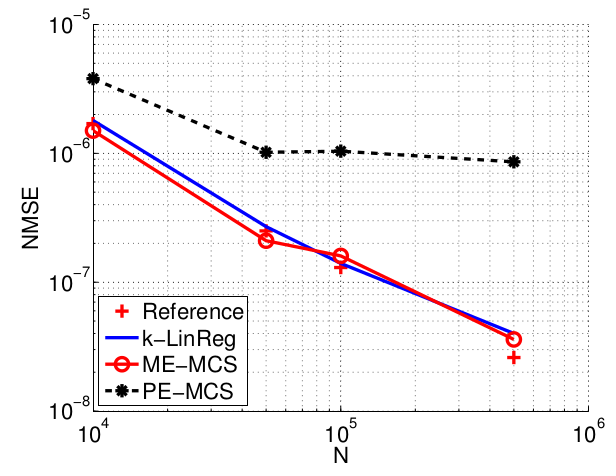
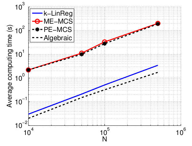
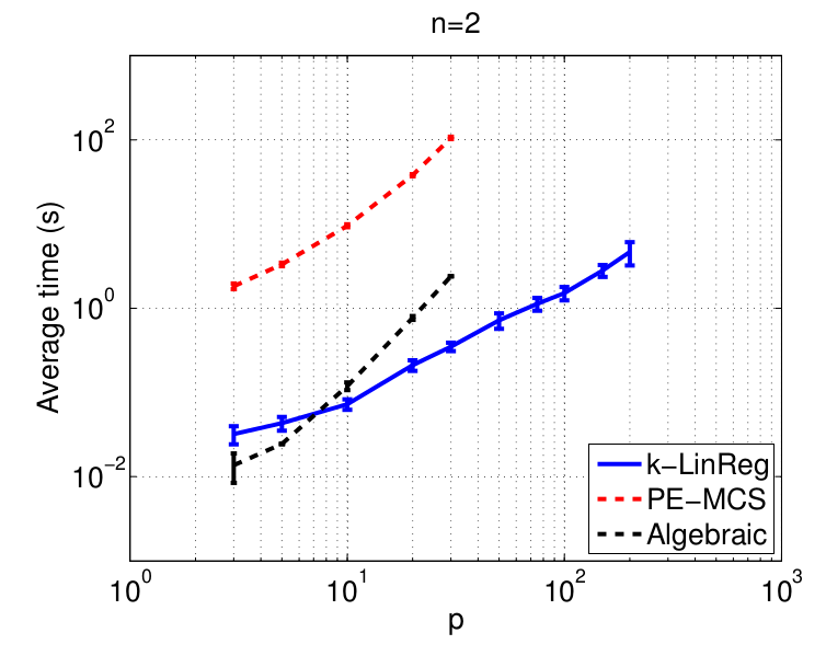
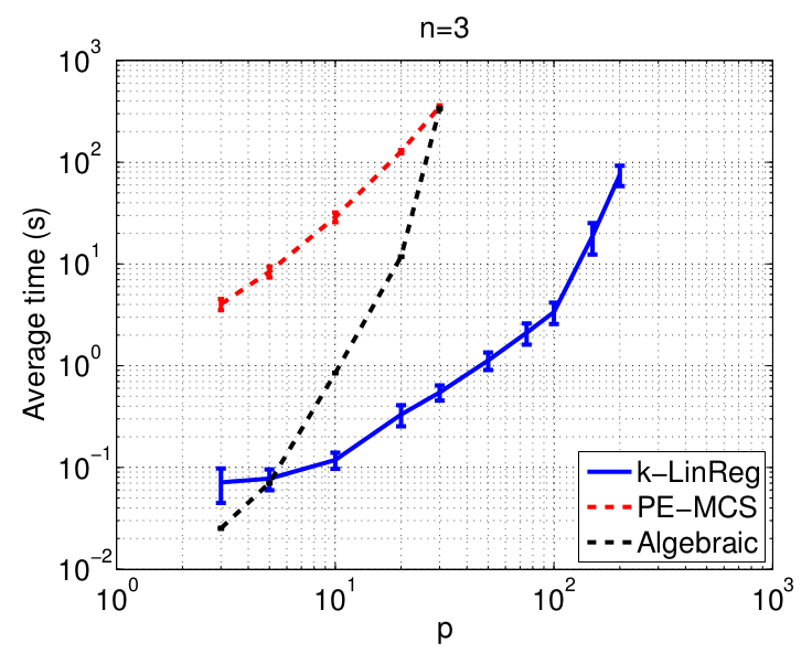
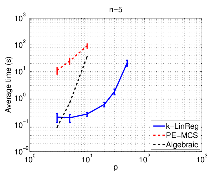
The figures below show the normalized mean squared error on the parameters (NMSE) and the average computing time (in seconds) of the methods with respect to the number of data N. These times are obtained with Matlab implementations of all methods running on a standard laptop.
Data in higher dimensions
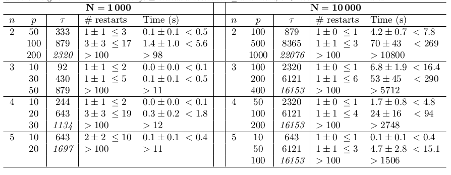
Global optimality
These experiments aim at testing the ability of k-LinReg to find the global optimum over 100 trials. With noiseless data, the optimum is 0 and global optimality can be easily checked by setting 'MSE < 1e-6' as a stopping criterion.
- C source code: test program generating the data, running the algorithm and printing the results
(also included in klinreg.tar.gz and compiled along with klinreg by running make)
- Example test with N = 1000 data points, n = 2 modes, p = 50 regressors:
	test_global 1000 2 50

	Expe = 1 / 100...  r=1, t=0.3614
	Expe = 2 / 100...  r=1, t=0.2771
	...
	Expe = 100 / 100...  r=1, t=0.2320
	************************
	 N = 1000, n = 2, p = 50
	 -> tau = 333
	 -> time = 0.0723 +- 0.0985 (tmax = 0.4954)
	 -> r = 1 +- 1 ( rmax = 3 )
	************************
The results show the number of restarts r and computing time required on average to reach the global optimum.
- More results
Hybrid dynamical system identification examples
In the following examples, the regression vector x is built from past inputs and outputs of a dynamical system switching between n modes (a so-called hybrid dynamical system).
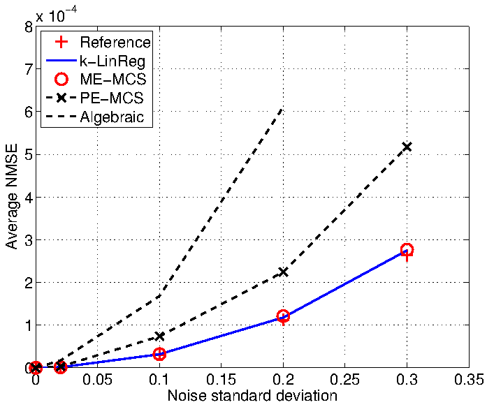
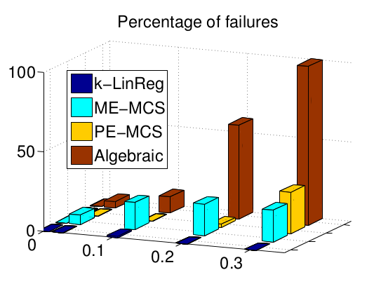
Robustness to noise
This example is taken from
R. Vidal, Recursive identification of switched ARX systems, Automatica 44(9):2274-2287, 2008,
and considers a system with n = 2 modes, a regression vector in dimension p = 2, and N = 1000 data points.
The figures show the influence of the noise standard deviation on the parametric error (NMSE) and the percentage of failures of the algorithms. The results of k-LinReg are obtained with a single restart (r = 1).
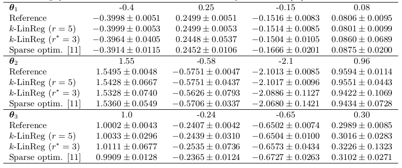
A slightly more difficult example
This example is taken from
L. Bako, Identification of switched linear systems via sparse optimization, Automatica 47(4):668-677, 2011,
and considers a system with n = 4 modes, a regression vector in dimension p = 4, and N = 300 data points.
The table shows the average parameter estimates over 100 trials with different noise sequences. The automatically tuned k-LinReg algorithm use r^* = 3 restarts and shows a performance comparable to the one of the sparse optimiztion method of Bako. However, the number of restarts needs to be slightly increased to r = 5 to cancel the difference between the k-LinReg average estimates and the ones of the reference model.
