A brief description of
WinSnoori
Yves Laprie
November 15, 2010
This page is not intended to present WinSnoori exhaustively but to demonstrate some of the facilities of WinSnoori which make its interest, or at least which can been exploited to solve some concrete problems. We will therefore present:
- how
to change
the initialization file
to adapt WinSnoori to your system configuration
- how
to use WinSnoori in an html page
- the
way of adapting the set of phonemes
to another language, and of organizing them so it is possible to explore
annotated corpora efficiently,
- how
to measure time and frequency
on the spectrogram,
- how
to get sharper harmonics
in spectrograms,
- what see
automatic speech recognition systems?
- how
to edit
speech files,
- the
advanced editing
tools that can be used to prepare
perception stimuli,
- how
to lower or raise formant and harmonic amplitudes with OLA
filtering,
- how
to use wav files
with chunks of annotations,
- the
automatic exploration of annotated corpora (phonetic
exploration or orthographic exploration)
- how
the Klatt synthesizer is interfaced,
- how
to modify speech rate and the fundamental frequency contour,
- how
to
correct the fundamental frequency contour easily,
- data journaling.
Changing the initialization file
The directoy where
WinSnoori is installed is the value of the registry
key HKEY_LOCAL_MACHINE\SOFTWARE\Wsno.
The
initialization file Wsno.ini in the Windows directory allows you to
adapt WinSnoori regarding messages, phonetic symbols
and font and audio player.
- SndRecorder is the player by WinSnoori
to play back signals synthesized by prosody editing tools. SndRecorder=C:\Winnt\system32\sndrec32.exe
is the default value. SndRecorder must be set
according to the windows system (Windows NT, Windows 95 or Windows 98).
- CountryFile contains the messages displayed by WinSnoori.
CountryFile=english.str is the
default value which corresponds to the file c:\Program Files\Wsno\Format\english.str. You can change messages by
editing this file or by replacing it with another file.
- LanguageFile is the file describing the set of phonemes. See Adapting the set of phonemes for further details.
- PhoneticFont is the font used to
display phonetic symbols. This font should be used according to the set of
phonetic symbols (see Changing the phonetic font).
Windows7: wsno.ini is in the virtual Windows folder named "AppData\Local\VirtualStore\Windows"
in the user folder, i.e. C:\Users\laprie\AppData\Local\VirtualStore\Windows for
me. This Windows 7 solution is intended to prevent users from accessing the
true Windows folder.
Using WinSnoori in
an Html page
You can launch WinSnoori
from a HTML page by adding the .wsn extension to any
valid sound file.
Here is
an example.
More generally you can run WinSnoori with the
following command :
wsno <file>
Adapting the set of
phonemes
Phonetic annotations belong to the set of phonetic
symbols used by WinSnoori. It can be useful to choose
another set of symbols, possibly not phonetic, to annotate some speech files.
With this aim in view the user is given the possibility to change the set of
phonetic symbols as well as the font.
Changing the set of symbols
There are already several sets of symbols in "c:\Program
Files\Wsno\format" :
- english.pho
(Timit symbols for english)
- englipa.pho
(IPA symbols for english and for the IPAPhon font)
- francais.pho
(SAM symbols for french)
- franipa.pho
(IPA symbols for french and for the IPAPhon font)
- frankiel.pho
(IPA symbols for french and the IPAKiel font)
These files contain the list of symbols, the
hierarchical phonetic menu, the phonetic classes, the hierarchical menu for
classes (this menu is used during exploration of annotated corpora) and the
first two formant frequencies for vowels (the frequency are used to plot
formants in F1-F2 plane). You can create a new file following the pattern
indicated in these files. For incorporating symbols not belonging to the
default font use "charmap" with the font
you want to use ("IPAPhon" font, for
instance), select symbols with "charmap"
and paste them in the new file. Note that these characters do not appear
correctly in the new file if you are using "notepad" to create the
new phonetic file. Anyway, WinSnoori will display
correct symbols. Note that the way you organize phonetic symbols into
phonetic classes influence the automatic exploration of annotated corpora. You
have to pay attention to define classes which take into account the manner and
the point of articulation of sounds.
Once this file is created,
modify the file "c:\Winnt\wsno.ini" (or in "windows" or
"windows95") accordingly. Assuming that the new file is xxxipa.phon replace the old line "LanguageFile=old.pho"
by "LanguageFile=xxxipa.pho". Do not forget
to modify the font so that symbols appear correctly in WinSnoori.
Changing the phonetic font
The first step is to check that the font is installed.
If it is not the case (especially for IPAPhon or IPAKiel font) install the font on your PC. Then, you can
modify the "wsno.ini" file by specifying the new phonetic font.
Assuming that the new font is "IPAPhon"
replace the old line "PhoneticFont=Arial"
by "PhoneticFont=IPAPhon".
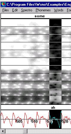
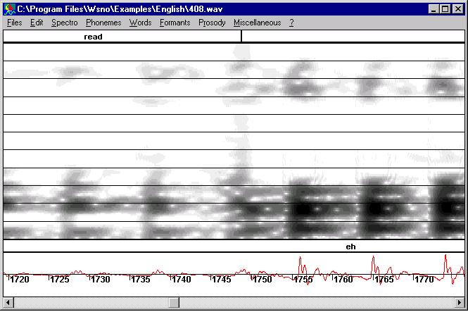
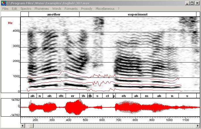
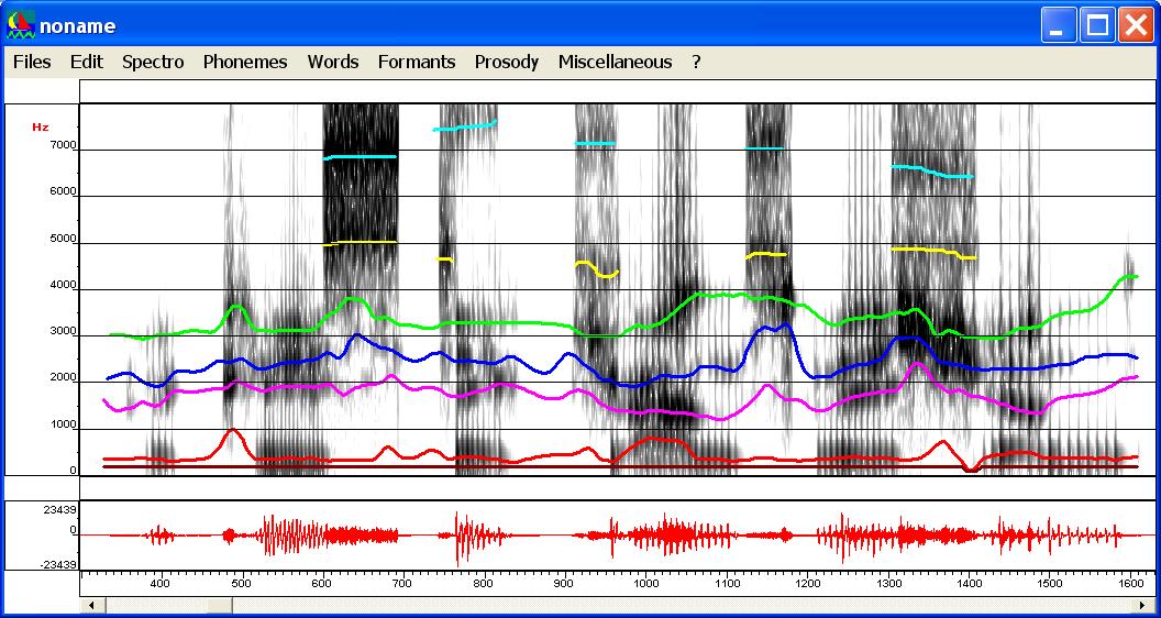
How to measure time and frequency on the spectrogram
Time and frequency coordinates pointed by
the mouse are indicated in the welcome window. Once the F0 has been calculated
F0 is also displayed. Besides the coordinates the duration of the highlighted
region is given in ms and in s-1. That information can be used to
evaluate F0 by hand, for instance.
|
|
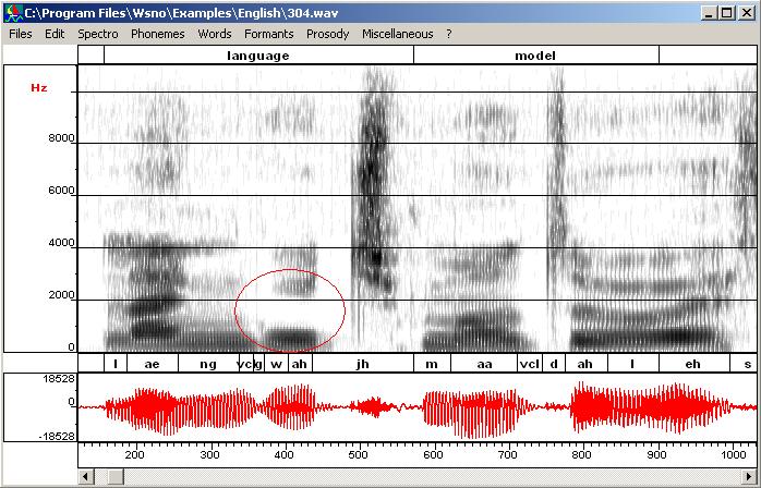
Suppose you have zoomed on the region displayed in
this spectrogram and you want to evaluate F0. You simply select a region
which obviously corresponds to the period of F0. When you point the mouse in
this region you obtain : |
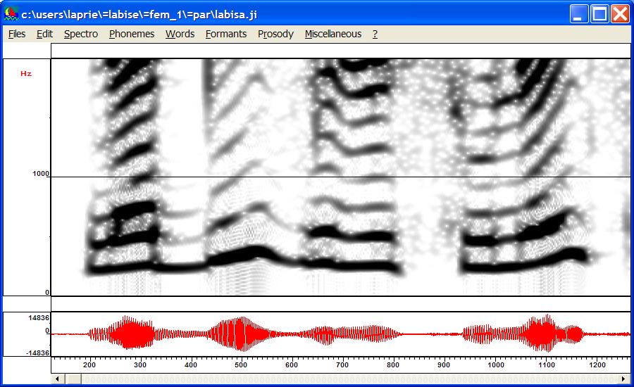
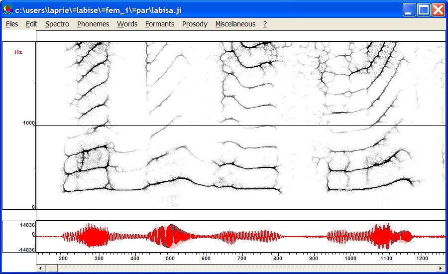
How to get sharper
harmonics in spectrogram
The reassignment algorithm proposed by F. Auger and P.
Flandrin, ("Improving the readibility
of timefrequency and time-scale representations by
the reassignment method," IEEE Transactions on Signal Processing, vol. 43,
no. 5, pp. 1068--1089, 1995) and used by Plante et
al. in speech processing (see the paper of Plante et
al. for further details (F. Plante and G. Meyer and
W.A. Ainsworth", "Improvement of speech spectrogram accuracy by the
method of reassignment", "IEEE Transactions on Speech and Audio
Processing", 6(3), pp 282-287, 1998)) enables sharper resolution in time
or frequency. If the window is small (4ms) the time
resolution is increased and enables the detection of glottal closure instants.
If the window is longer (32 ms for instance) very fine harmonics are obtained.
The first image is a narrow band spectrogram of a female voice,
the second is the corresponding reassigned spectrogram.
|
1
|
|
|
2
|
|
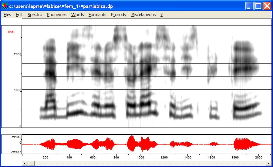
What see automatic speech
recognition systems?
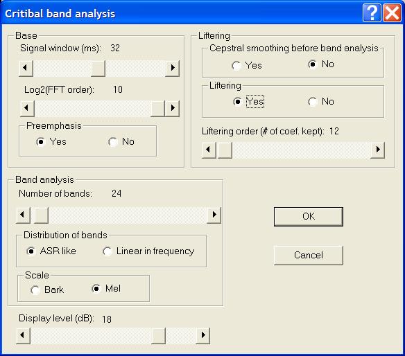
The "Critical bands" option in the
spectrogram menu and the corresponding option spectral slice allows you to get
a better idea of what spectral data automatic speech recognition systems use.
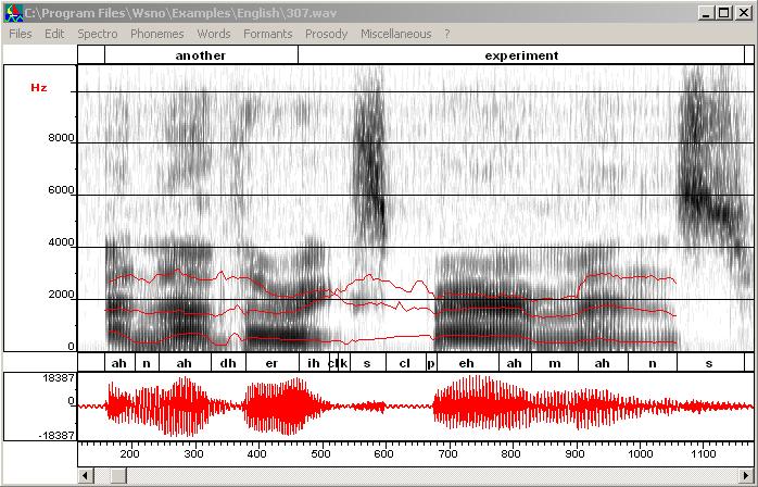
The next image shows the spectrogram of a female voice processed by mel filters displayed in the mel frequency scale. Note that the DCT has not been
performed. This explains why first harmonics remains. On the contrary, there is
a strong smoothing in high frequencies and their contribution is weaker than
with a linear frequency scale.
|
1
|
|
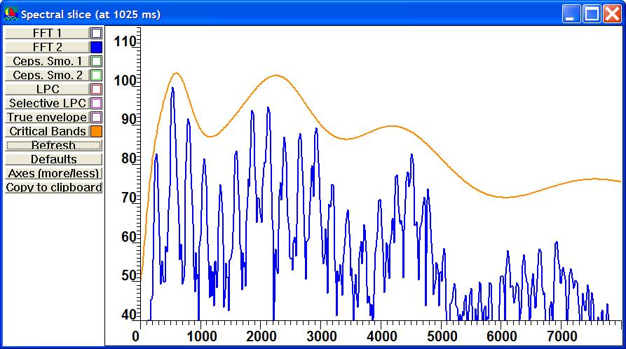
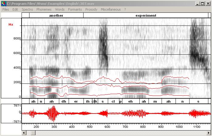
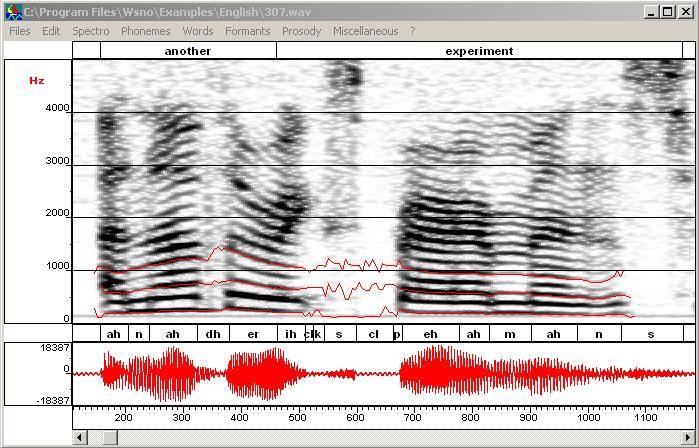
The fllowing images shows the spectral slice which has been obtained with
mel cepstral smoothing. Unlike standard mel cepstral analysis an IDCT-III
transform has been applied to mel cepstra
to recover a spectrum. Two extra triangular filters (one at zeo
Hz and one at Fs/2) have been added to keep the energy of the spectrum. This image correspond to standard parameters used in
automatic speech recognition, i.e. 24 filters, 12 coefficients.
|
|
|
How to edit speech files
The editor of WinSnoori
is not intended to make modifications on large portions of signal since the
window is limited but to edit signal by taking into account the acoustical
effects of the editing commands. We describe two situations :
- you have created some artificial discontinuity in the signal and
you want to remove it,
- you want to filter the signal to remove some acoustic cue.
Note: The editor of WinSnoori
can handle files of any size. Nevertheless the duration of the window is
limited to 4 seconds in order to minimize the memory required by WinSnoori. This means that if you want to perform editing
commands on large portions of a file you may be obliged to iterate your command
on small portions of the file to be modified.
Suppressing a discontinuity (spectral bar or
click)
|
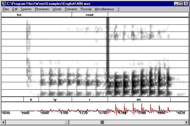
When you cut a region you run the risk
of breaking the periodic structure of speech which gives rise to
discontinuities. These discontinuities correspond to spectral bars in the
spectrogram and "clicks" when your are listening to the signal. The following figure
exhibits such a discontinuity. You can listen to this discontinuity here. |
|
|
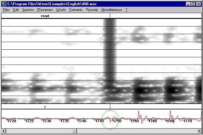
You can suppress or at least reduce the influence of
this discontinuity by restoring the periodic structure of speech. First, zoom
in the signal in order to localize the discontinuity (at the center of the
green circle). Choose a reasonable zoom so that the periodic structure does
appear. |
|
|
Then cut a portion of signal so that an artificial
periodic structure is restored. Recompute the spectrogram
if need be. |
|
|
This figure shows the final signal. Here is the new signal without
"click". |
|
You can also
create artificial bursts when you cut a signal portion at a voicing
onset. In this case you can remove this artificial burst be
"damping" the signal. Use "damp left" when the burst
appears at the voice onset or the "damp right" when the burst
appears at the end of a voiced region.
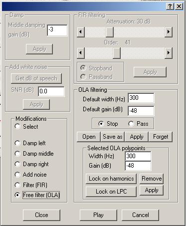
Editing tools
|
The "Editing tools" window enables
attenuations (left, right, middle), the addition of noise, filtering through
FIR and OLA filters. You have to choose among these several possibilities.
Here, the OLA filtering has been selected. As it is shown below its enables filtering along time
x frequency trajectories. This
window can be called from
the "Edit" menu. |
|
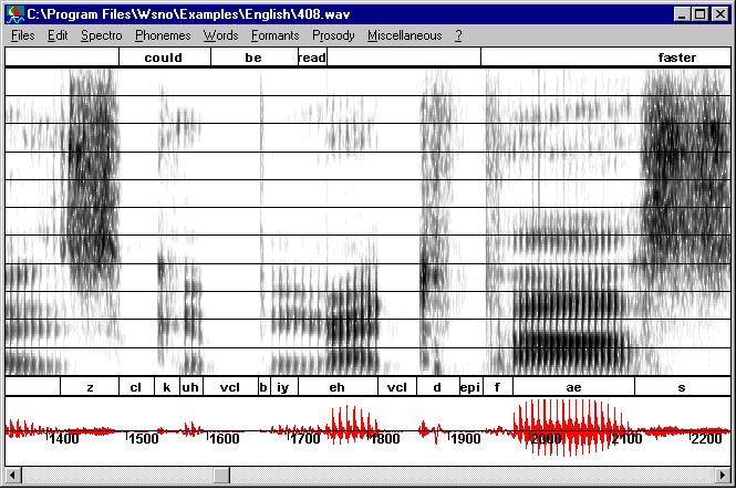
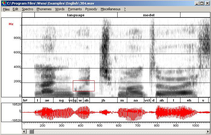
Filtering a time x frequency region
Suppose you want to investigate the
importance of some cue (burst or formant trajectory for instance). One solution
could be to remove this cue from signal by filtering.
Here is an example on the
file c:\Program Files\Wsno\Examples\English\404.wav.
Suppose we want to remove F2 information in the sound "ah" of
language. Call "FIR Filtering" from the Editing
tools window (edit menu), select "Stop band" instead of
"Pass band", set the filter order to 61 and
the attenuation to 35 dB. Then, define the region to be filtered by dragging
the left button and click the "Apply" button. As filtering has may
create a small discontinuity you probably have to remove it (it is the case
with this example). Here are the original and the final spectrograms.
|
Original (sound and spectrogram) |
Lowering or raising formants and harmonics by OLA
filtering
Editing formant amplitudes
|
|
The second step is to apply the filters corresponding to
these trajectories.
|
|

|
|
Editing harmonic amplitudes
|
|
|
|
How to use wav files
with chunks of annotations
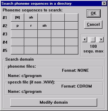
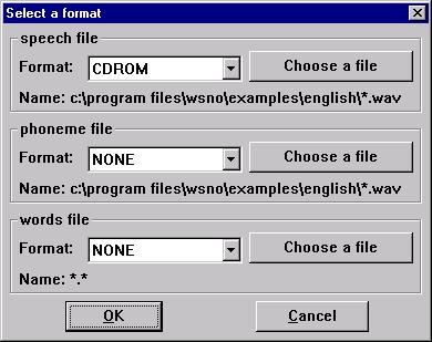
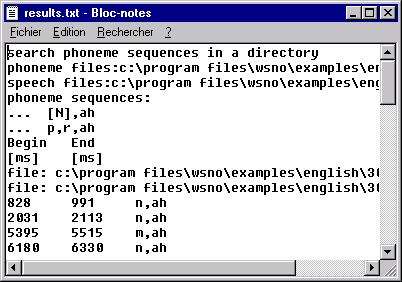
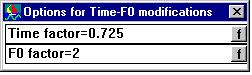
Automatic exploration of annotated corpora
Searching for a phoneme sequence
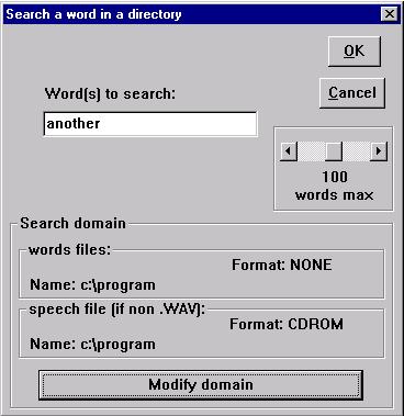
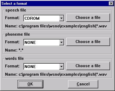
Searching for the occurrences of a word
|
As for phonetic
exploration, you specify the word to be searched for, "another" for
instance. |
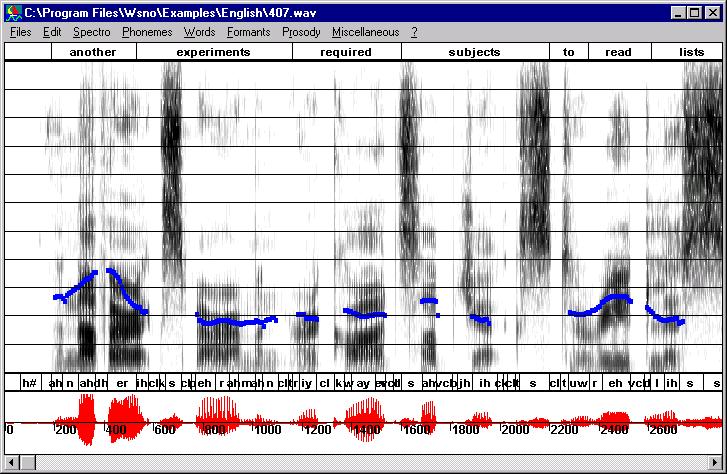
Graphical interface for the Klatt
synthesizer
- First, compute LPC roots on this word and use
"Keep decoration" in the Spectro menu
to attach the display of LPC roots to the spectrogram image. This first
step is necessay if you don't want to use the
automatic formant tracking.
- Enter the graphical interface (opening this
window takes a few seconds because F0 is computed for the whole file).
- Here you have the choice of getting formants by
automatic formant tracking or by drawing them by hand.
- Automatic formant tracking: launch the
automatic formant tracking (select the region you want to process and use
"Copy synthesis/Formant tracking/Tracking from scratch").
Automatic formant tracking only tracks F1 to F4. At this point you should
obtain this result.
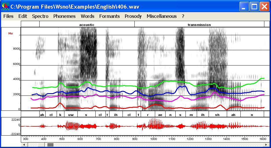
You have to draw F5 and F6 by hand if you want to add them (see next item). - By hand: draw formants
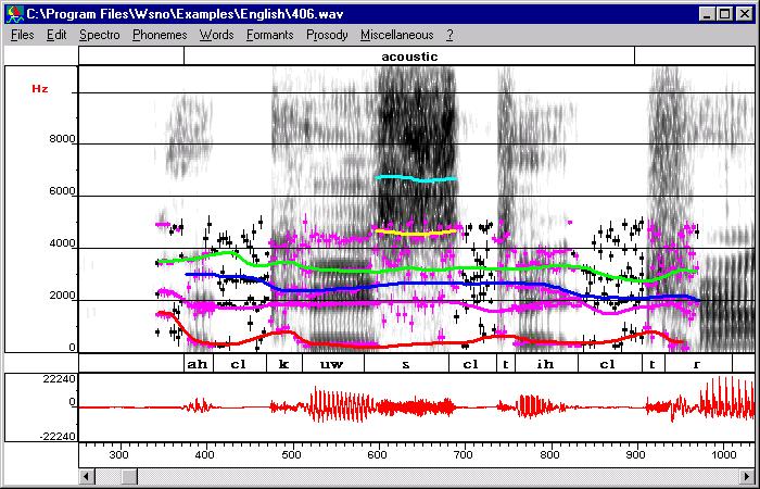
trajectories F1, F2, F3, F4 everywhere, and F5, F6 for fricative
segments. You are not obliged to draw very accurate trajectories since
you can automatically put the trajectories close to the LPC tracks. At
this point you should obtain such a result.
The synthesized signal looks awful, at least because the prosody has not been incorporated and trajectories are too rough. The next step consists in registering trajectories. For that purpose select trajectories to be registered, (CTRL+left click on these trajectories) and use "Register with cepstral smoothing" in the "Copy synthesis" menu. Trajectories can be edited in order to remove chaotic points in low energy regions or to correct trajectories where two formants are close together or don't correspond to any spectral peak. - Then get the F0 information (Copy synthesis/Get
F0) and go back to the frequency scale (Scale/Frequency) to see formant
trajectories.
- Then adjust the formant amplitudes by using
"Copy synthesis" from the "Copy synthesis" menu.
Amplitudes are adjusted only for formant trajectories selected. If you
want to adjust all the trajectories use "Select/All" before the
copy synthesis. This function adjust only
amplitudes of formants for the parallel branch. Note that the resulting
curves are not smoothed. Smooth them to eliminate small jumps. Note that
the first harmonics are modified by using the nasal formant as proposed by
J. N. Holmes (Speech Communication, Vol 2. pp
251-273, 1983). With this simple scenario you should obtain these formant
trajectories (Klatt file) and
this synthesized waveform.
Modifying the speech rate and the fundamental frequency
contour