
Update 17/12/2020 : Since the publication of this post, a group of French researchers has created a website gathering recent publications and news articles on the use of group testing for COVID-19 detection around the world. Check it out! https://www.groupool-covid19.org/
Now that a large part of the world’ population is in lockdown to fight against the global spread of the new coronavirus, the crucial question is: What’s next? As lock-down measures will progressively be lifted, the key to avoid second and third waves of the pandemics will be massive and rapid testing, combined with case tracking and targeted quarantining. Unfortunately, the testing capacity of most countries is currently not nearly enough.
Last week, researchers at the Frankfurt Red Cross Blood Donor Service and the Institute for Medical Virology at the University Hospital Frankfurt of Goethe University succeeded in developing a procedure that makes it possible to immediately and dramatically increase worldwide testing capacities for detecting SARS-CoV-2, the virus behind COVID-19. The procedure is based on pool testing (also called group testing), a principle as genius as simple, that was already used to detect syphilis during WWII. Rather than analysing individual patients’ samples (usually swabs from the throat or nose), one mixes a bunch of samples together, say 8, and runs the test on this cocktail, called a mini-pool. If the result is negative, you can reliably conclude that none of the 8 patients were infected, from one single test! If the test is positive, just divide your samples into two groups of 4 and repeat, until either a negative result is reached or a single sample is left.
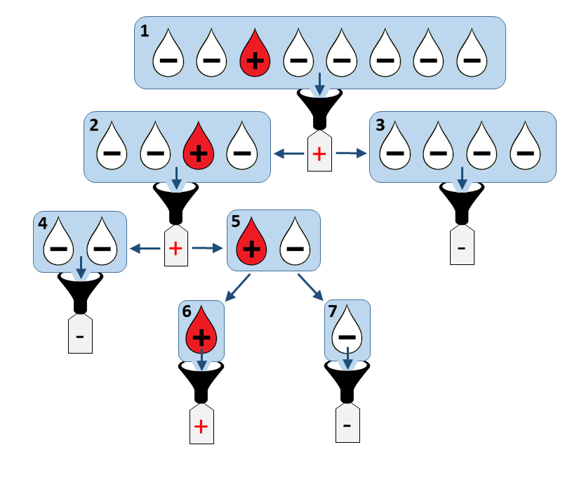
This procedure could readily be implemented by any laboratory in the world without the need for extra equipment. Given that running a single PCR test for COVID-19 takes several hours on dedicated machines, cutting down their number could save precious time in the ongoing fight against SARS-CoV-2.
But how much time exactly? The figure below shows the theoretical average number of test per sample needed using group testing as a function of the population’s infection rate for different mini-pool sizes:
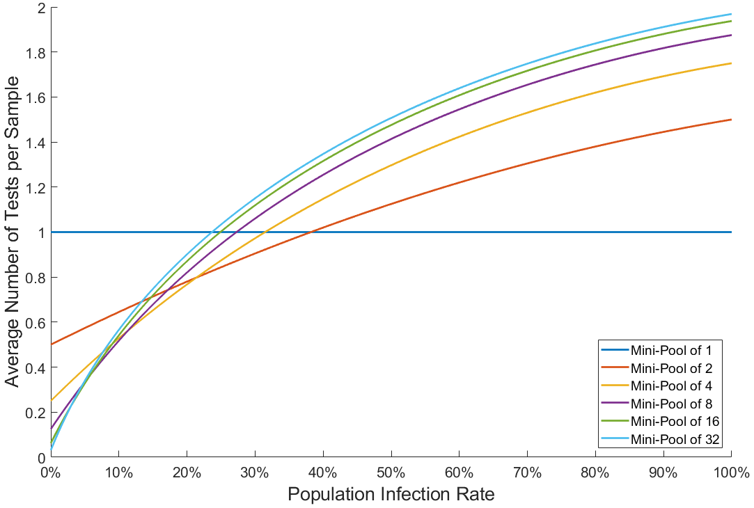
Note that using mini-pools of size 1 corresponds to classical testing: one test per sample. The graph shows that if the proportion of infected people is larger than about 25% in the tested population, group testing is not advantageous compared to conventional testing. However, in a scenario where large campaigns of tests are conducted on random people in cities in order to track and isolate positive cases, it is reasonable to assume that no more than 10% of the population will be infected by COVID-19 at any given time. Here is a zoomed version of the above graph for infection rates below 10%. We also show on the right the inverse of the graph, which represents the average speed-up brought by group testing:
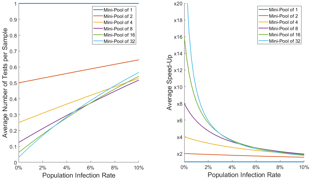
We see that for infection rates around 5%, using mini-pools of 4 already boosts testing capacities by a factor of 2.5, while for infection rates around 1% mini-pools of 16 may speed up tests by a factor of 10 or more ! It is also interesting to note that for infections rates above 6%, using pools of more than 4 samples does not significantly improve results.
Deriving the formulas for those graphs is actually a quite fun maths problem! In the rest of this blog post, I will try to explain how to do it in an accessible way. My goal is to provide an example of interesting and useful maths exercise to enjoy during lockdown. I also secretly hope that it can help raising awareness in group testing, which does not seem to have received a lot of attention as of yet by politicians or media. Let’s spread the word together!
1. Hypotheses
First, we will assume that each test can detect a positive sample inside a mini-pool with 100% accuracy (no false positives or false negatives). The German study on SARS-CoV-2 mentioned earlier showed that mini-pools of 5 samples can be used without degrading accuracy. This recent paper from the Israel Institute of Technology and the Rambam Health Care Campus (Haifa, Israel) suggests that pools of up to 32 or even 64 samples could be used while keeping the false-negative rate relatively low. Amplification cycles (running multiple tests) can also be used to improve reliability, but this will not be investigated here.
Second, we will suppose that all samples have the same independent probability P+ (between 0 and 1) of being positive, representing the population’s infection rate. Note that this independence assumption does not hold if we test, e.g., a group of people leaving in the same house. Here, we assume that samples are taken uniformly at random in an infected population.
Finally, for the sake of exposure, we will only consider mini-pools of size N where N is a power of 2, e.g., 23 = 2 x 2 x 2 = 8. This will make computations easier and cleaner.
2. Worst-case number of tests
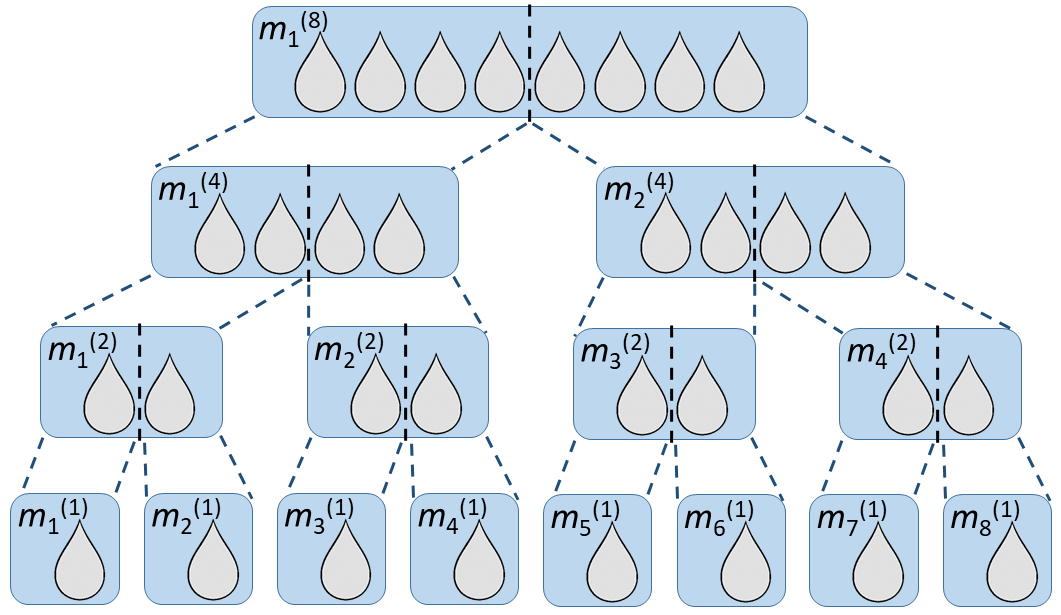
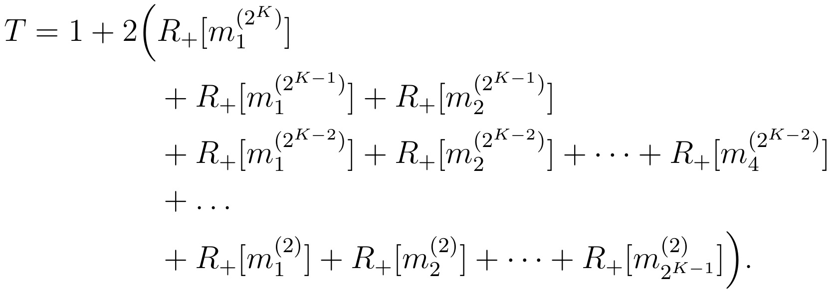
As a warm up exercise, let us find what is the maximal number of tests Tmax needed to analyse an initial mini-pool of N=2K samples. This corresponds to the « worst case » where every mini-pool along the procedure is tested positive and hence has to be split into two and further analysed. An example of this situation is illustrated below:
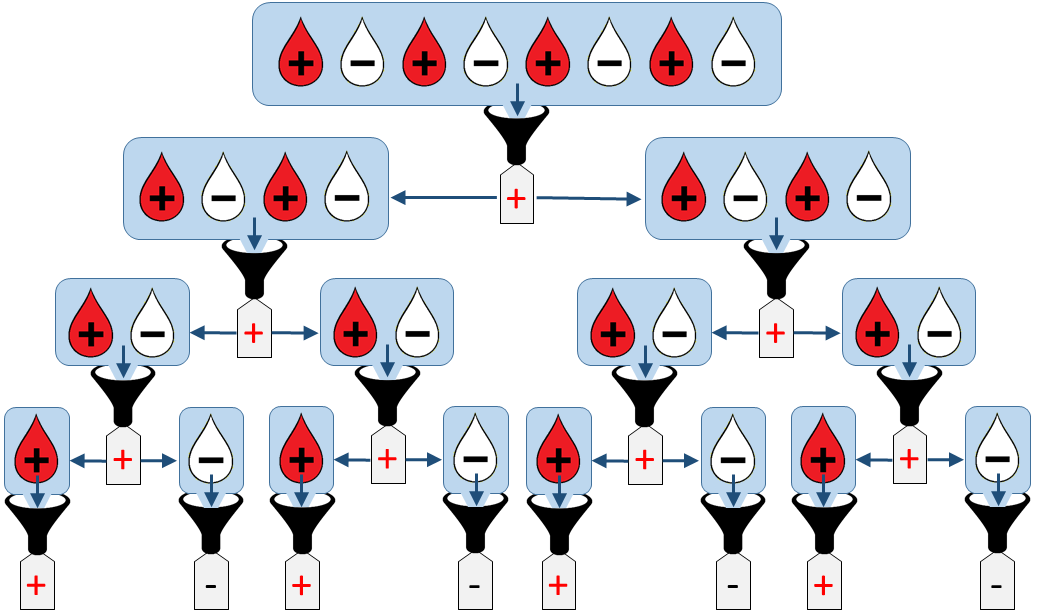
By counting the number of positive mini-pools of size >1, we see that:
![]()
Using the formula for sums of geometrical series, we obtain:
![]()
Shoot, in the worst case, we have to run more tests than when simply testing the N samples individually! Is pool-testing really that good after all?
Well, it all depends on how often this worst situation happens. To get an idea of this, let us stick to the example of Figure 2 where exactly half of the samples to be tested are positive. Then, the worst case only happens when the samples are precisely in the alternated order +,–,+,–,… The probability of this to happen is the number of alternated orderings divided by the total number of orderings:
![]()
To order N samples, there are N ways of choosing the first one, then (N-1) ways of choosing the second one, (N-2) ways of choosing the third one, etc. The total number of orderings is hence N x (N-1) x (N-2) x … x 1 = N! (« N factorial »). To order them alternately, there are (N/2)! ways to order positive samples and (N/2)! ways to order negative samples, hence (N/2)! x (N/2)! = ((N/2)!)² ways in total. We obtain:

where we used the following combinatorics notation:
![]()
pronounced « n choose k ». This counts the number of ways of placing k identical elements into n available positions. Here is a summary of our results for different values of N:
| Initial mini-pool size N | Maximum number of tests Tmax | Probability Pworst (for 50% infection) |
| 2 | 3 | 1/2 |
| 4 | 7 | 1/6 |
| 8 | 15 | 1/70 |
| 16 | 31 | 1/12,870 |
| 32 | 63 | 1/601,080,390 |
As can be seen, the worst case happens very rarely when using sufficiently large mini-pools. That’s reassuring!
3. Average number of tests
Let us now look at the more general problem of the average number of tests needed when using mini-pools of size N, for a given infection rate P+. To tackle this we will need to introduce appropriate notations (which is often the most difficult part of real-world maths problems). We will denote by m(i) a mini-pool of i samples, i.e., a pool of i. The mini-pools of a given size will be numbered « from left to right », as shown in the example below:
With this notation, the individual samples are hence written as pools of 1, that is, m1(1), m2(1), … , mN(1). We will use R+[m(i)] to denote the positivity of a pool, where R+[m(i)]=1 if m(i) contains a positive sample and R+[m(i)]=0 otherwise. Similarly we will denote by R–[m(i)] = ( 1 – R+[m(i)] ) the negativity of a pool.
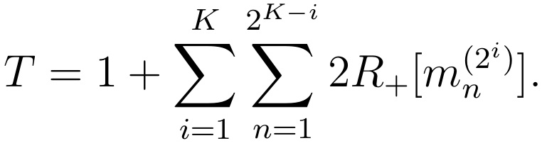
When doing a group test, we first need to test the initial mini-pool containing all samples. Then, whenever a mini-pool is tested positive, we split it into 2 pools of equal size and run further tests on them. A first approach to estimate the number of test needed is hence to count twice the number of positive mini-pools of size 2 or more. Following our notations, this gives:
This can be written in a more compact way using the mathematical symbol for sums:
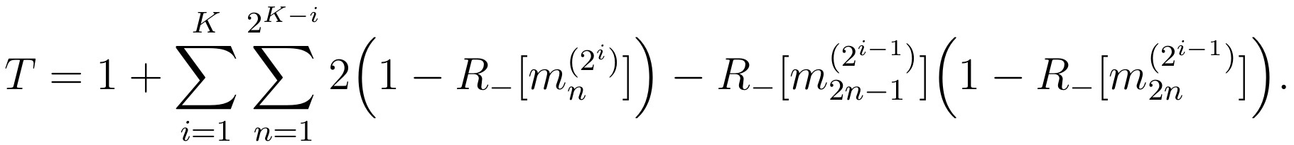
However this formula is missing « shortcuts », such as the one showed in Figure 1. When a mini-pool is tested positive, if the first half of it is tested negative, then there is no need to test the second half: we know it must be positive. To remove these shortcuts in our count, we need to correct the above formula as follows:
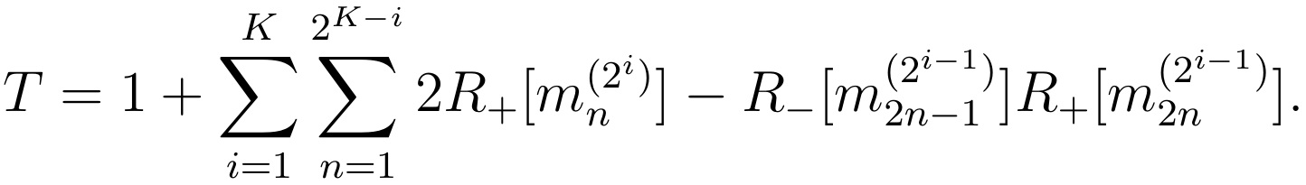
The new term removes one test whenever the first half of a pool is negative while the second half is positive. For what follows, it will be convenient to rewrite this formula only in terms of the negativity of mini-pools:
We now want to know how much T will be in average, given that each individual sample has a probability P+ of being positive. This quantity is called the « expectation of T » and we note it E{T}. Using the fact that the expectation is linear and that the expectation of the product of two independent variables is the product of their expectations, we have from the previous formula:

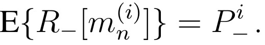
We are left with the problem of computing the expectations of the mini-pools’ negativities. By our hypothesis, a single sample is negative with probability P–=(1-P+). Hence, we have:
![]()
for any n between 1 and N. In addition, a mixture of i samples will be tested negative if and only if every sample in it is negative. Its expected negativity is hence the product of the expected negativity of each sample, i.e., (P– ) x (P– ) x (P– ) x … This gives:
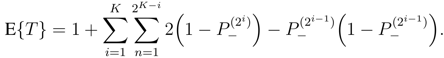
Inserting these in the previous expression of E{T} we obtain:
After simplification, we finally obtain the following general formula for the average number of tests:
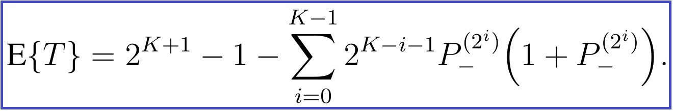
It is also convenient to express the average number of test per sample. To do this, we divide the above expression by the initial size of the mini-pool, N=2K:
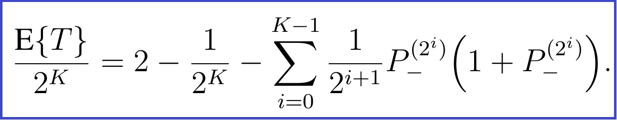
This expression is a polynomial in P–. As expected, we see that if the population is 100% infected (P– = 0), pool-testing requires about twice as many tests as the regular procedure (the « worst-case » situation studied in the last section). We also see that the number of needed tests decreases with the infection rate, as showed in the graphs at the beginning of this post.
Here is a table detailing mean numbers of tests per samples as a function of infection rate and initial mini-pool size:
| Infection rate ► ▼ Initial mini-pool size |
0.5% | 1% | 2% | 3% | 5% | 8% | 10% | 20% | 50% |
| 2 | 0.51 | 0.51 | 0.53 | 0.54 | 0.57 | 0.62 | 0.64 | 0.78 | 1.12 |
| 4 | 0.26 | 0.28 | 0.31 | 0.34 | 0.39 | 0.48 | 0.53 | 0.77 | 1.30 |
| 8 | 0.15 | 0.17 | 0.21 | 0.25 | 0.33 | 0.45 | 0.52 | 0.82 | 1.41 |
| 16 | 0.09 | 0.12 | 0.18 | 0.23 | 0.33 | 0.46 | 0.54 | 0.87 | 1.47 |
| 32 | 0.07 | 0.10 | 0.17 | 0.23 | 0.34 | 0.48 | 0.57 | 0.90 | 1.51 |
4. Open questions
There are still interesting open questions left to explore. In particular, if the tests are not 100% accurate, what is the best way to reduce errors using multiple cross tests? How to generalise these formulas to initial pools which are not powers of two? I leave these questions to the interested readers, and maybe I’ll come back to it in a future blog post!
Stay safe everyone!